A common task – Get and sort a list of tasks that are not yet due according to due dates
Got the following question:
Suppose on column A I have entries and on column B i have due dates for the entries. Is it possible to have excel automatically rearrange the ROWS such that the nearest dates appear at the top and the furthest dates at the bottom? Thank you in advance
First thing on my mind: This can be done easily by sorting column B in ascending order.
Then I stop and rethink… maybe the reader wants to list the tasks that are not yet due… and probably on a separate table. And even more, new tasks with new due dates will be added from time to time and Excel should be able to get him updated list of tasks not yet due “automatically”… That makes sense and I believe it’s a common task for many people.
The following screen cast visualize the request:
And this is achieved with a simple helper column + Pivot Table. Here’s the step by step instruction:
You may download a to Sample File – Sort Task according to due dates to follow along.
Let’s start with a list of 10 tasks (note: I did the following screenshots last week, so let’s assume today is Dec 2, 2017)

1. Turn the range into an Excel Table.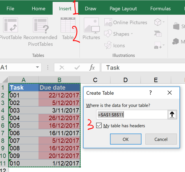
2. Add a helper column
In C1, input “Days to due”, then you will see the table expand automatically.

3. Input a simple formula to show number of days to the due date.
In C2, input “=”, then press left arrow key once (or use your mouse to point to cell B2), you will see the formula changed to [@[Due date]] automatically. Don’t panic! This is a wonderful feature of Excel Table. Simply continue the formula with “– today()“. You will see the same formula “[@[Due date]] – TODAY()” filled the column automatically.

To make the results look more meaningful to you, change the format to “General”.

4. Insert Pivot Table.
Follow the steps shown below. Note before you insert PivotTable, select any cell into the Table, then you will see Excel detects the Table name correctly for you. For easy reference, let’s place the PivotTable to E1 of the same worksheet.

Move the “Task” and “Days to due” to Rows and Value respectively.

As this point, you will see a PivotTable that is basically the same as the original table.

Since we want to focus on tasks that are going to due, i.e. “Days to due” > 0, we can filter the Pivot Table as follow:

Note: We can do a few tricks here depending our needs. If we want to include task that is due on current day, filter “Great Than Or Equal To 0” instead. If we want “overdue” tasks, we may filter “Less Than 0” here.
Now you should get the following:

Sort the “Sum of Days to due” A to Z

Now the result is basically what we want. (Tip: You may rename the column header)

To make the result more reader-friendly, I would put “Due date” to Rows (under Task).

By default, PivotTable is shown in Compact Form. Let’s change it to “Tabular Form”.

Remove all “Subtotals”.

Remove the automatically added “Months”.

Note: If you are using Excel 2010, you won’t have the “Months” added by Excel so that you won’t need this step. (Not sure about 2013 as I have never used it ;p )
Finally remove “Grand Total”

5. Here we go

Wait… What if I have new tasks added to the list?
One of the beauties of Excel Table is automatic expansion: When new data are added to the bottom of the table, the formula in Column C will fill in automatically. On top of it, do you remember that the Pivot Table was created using the Table name, not range, as the source. That means the Pivot Table will get the expanded range as the source. Simply put, you don’t need to worry about updating the Pivot Table source every time it is updated.
See it in action:
Make sense?
Well… it’s not 100% automatic as you will still need to “Refresh” the pivot table every time you have new data added.
To go one more step “closer” to “fully automatic”, we may instruct Excel to refresh that Pivot Table when opening the file.


Hope you like it.
Do you handle this task by using Macro or other methods? Please share with us your thought.


