Answer to the 5 little Tricks posted in the beginning of the year – Part 1/5

Transpose Data – Result is static

This is actually a simple trick of using Copy and Paster (Special, Transpose).  See? It can be done in a second.

Nevertheless, as I mentioned in previous post, many people are not aware of this simple trick even though they work with Excel every day (they work in accounting field).  What they did was to move cell one by one… @_@

Here’s the step-by-step screenshot:

1. Of course is to Copy the source table
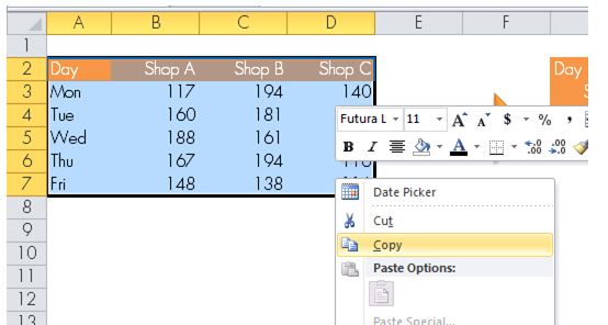
2. On destination cell, right-click –> Click on the “Transpose” icon directly. (Note: The icon appears as the fourth icon under the Paste Options; and also under Paste Special Options:

   

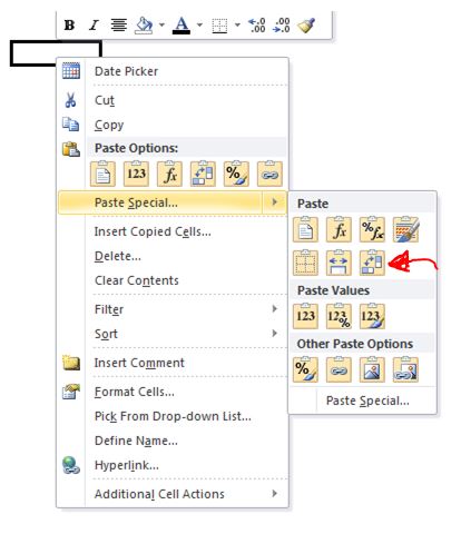
3. Just in case you like to go into the Paste Special menu:
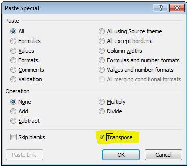
4. OK.

This is the easiest way to transpose a table (rows to columns, columns to rows).  However the result is static, meaning the data do not change with the data in the source table.

Transpose Data – Result is dynamic, i.e. linked

In order to make a linked transposed table, we need formula.  There is a TRANSPOSE function indeed.

However there are few tricky points to use TRANSPOSE:

First, it is an array function, meaning you have to press Ctrl+Shift+Enter to input the formula.  Second, also the most tricky one, is you have to select an exact transposed area in order to transpose the content successfully.

E.g. If the source table is a range of 4×6, then you should select a range of 6×4 in order to make it work.  Imagine a table of 26×128, is it that easy to select a range of 128×26?  @_@

To tackle this cumbersome step, here’s my tip:

1. Do the Copy and Paste (Special, Transpose) as demonstrated before.
2. Right after the Paste, while the resulted range is still highlighted, type =TRANSPOSE(array), then Ctrl+Shift+Enter

Now you have a transposed table that is linked to the source table.

Is it much easier?  🙂

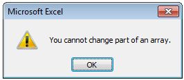
Nevertheless, another tricky point about TRANSPOSE is you cannot edit part of the resulting table (array).  If you try to insert, remove, or simply delete a cell of the resulting table, you will see this error message:

This could be annoying to many users.  So let’s explore another way of doing the same without using the TRANSPOSE function.  What we need is just a few more steps that can be done within a minute indeed.

1. Copy and Paste (Special, Link) to create a “helper” table

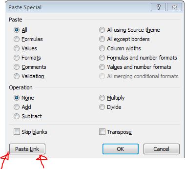
(Tip: you may do it on the right-click menu directly, look for the “Link” icon that is the rightmost icon under Paste option)

2. While the “pasted” table is still selected, press Ctrl+H to open the Find and Replace dialog box, Find “=” and Replace with “^=” (note: do not enter the quotation mark)

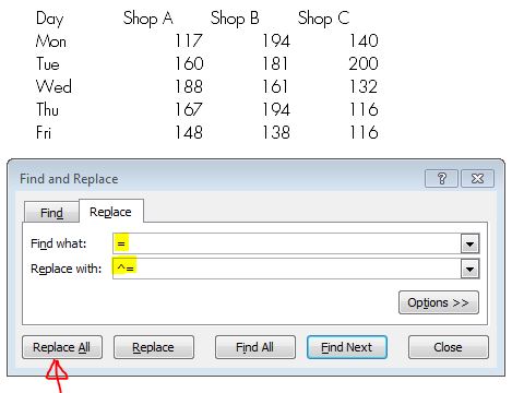
You should be able to see the result like this: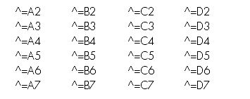

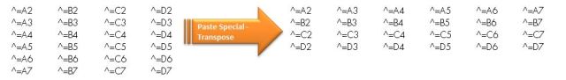
3. Now do the Copy and Paste (Special, Transpose) step

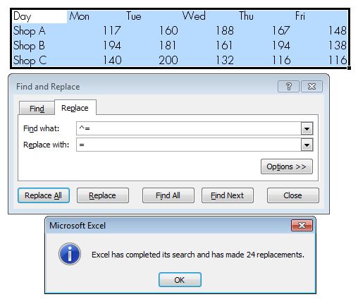
4. Repeat the Find and Replace, but in reverse way.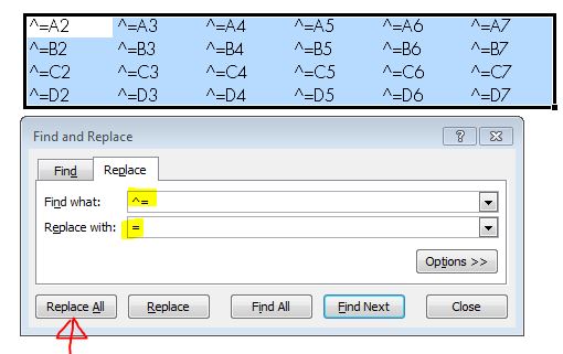

5. Here we go!

An animated GIF for easy reference:

As simple as this! 🙂