SUMIF is a handy but helpful function.  The syntax is simple:

=SUMIF(range,criteria,[sum range]

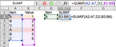
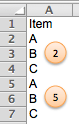
What it does is quite straight forward indeed.  In the example above, it instructs Excel to look into the range (A2:A7), look for the matching criteria, which is “A“, and then sum the “corresponding” value in the sum range (B2:B7).  That’s how we get 5 as a result.  Make sense?

However, if we point to incorrect reference for sum range, SUMIF may give you an unexpected (and also incorrect) result.  What do I mean?  Let’s say if I mistype (by human error of course) the formula to

=SUMIF(A2:A7,D2,B3:B8) 'Note the one cell shift in the sum range

Do you expect a result of 4? 

Surprisingly the result is 7.

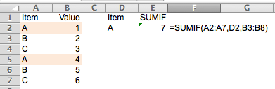
You may wonder HOW?

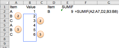
Now let’s look at another example.  What if I keep the same “mistyped” formula but changed the criteria in D2 to “B”.

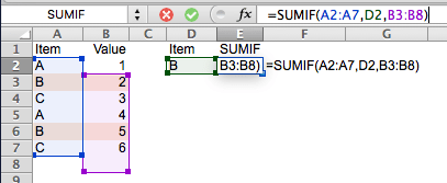
Do you expect 7 as a result?

Yes. I do.  But Excel returns 9.

So what happened?  Is it a bug?

No.  It’s a feature indeed. 🙂

Below is an official “remark” for the function SUMIF:

The sum_range argument does not have to be the same size and shape as the range argument. The actual cells that are added are determined by using the upper leftmost cell in the sum_range argument as the beginning cell, and then including cells that correspond in size and shape to the range argument.

Full description at https://support.office.com/en-us/article/SUMIF-function-169b8c99-c05c-4483-a712-1697a653039b

What?  “Does not have to be the same size and shape“?  What is “upper leftmost“?  What is “correspond in size and shape…“?

Let’s illustrate it using our example:

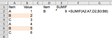
=SUMIF(A2:A7,D2,B3:B8)

For this formula, Excel first looks into the range A2:A7 for a match to D2 (“B”).

Where are the matches?  They are the 2nd and 5th position of the range.

Now Excel goes to the argument set for sum range (B3:B8), which is essentially B3 (the upper leftmost), then determines the “actual” sum range by setting a range of “correspond in size and shape” from B3, i.e. B3:B8 because the original range Excel looked into is a 1D vertical range consisting of 6 cells.  (Try: change the sum range to B3:B4)

And now is the tricky part: Excel adds the value in the “corresponding” position(s), i.e. 2nd and 5th values, in the sum range, which are 3 and 6 respectively.

Now it makes sense that SUMIF returns the result of 9, instead of 7.

Put it in other word, the range and the sum range do not necessarily sit together side by side.  You may arrange your data in the following way to have SUMIF worked…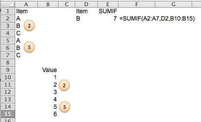

although it is not “human-friendly” at all.

Wait… it is so confusing, isn’t it?  Why Excel has such “feature” for SUMIF?

Because it gives you the flexibility to perform dynamic SUMIF.

Anyway, I guess most people do not appreciate this “feature” of allowing different size and shape of the sum range from the range, and it is no longer available in SUMIFS.

Having said that, you still need to pay attention to the “position” of the sum range,

=SUMIFS(B3:B9,A2:A8,D2)

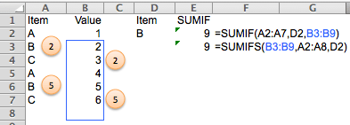
as both SUMIF and SUMIFS are following the same logic in a way… 😛