If you do Pivot Table, I believe you should have experienced the following too.  

GETPIVOTDATA is good.  But sometimes we just want a simple cell reference.  We may disable the GETPIVOTDATA easily by going to Pivot Table Option –> Uncheck the “Generate GetPivotData”:

But as I said, GETPIVOTDATA is good.  I want to keep it on.  So here is a simple trick I would do.

Instead of selecting a single cell that you want to refer to, select just one more cell.  See the screenshot below: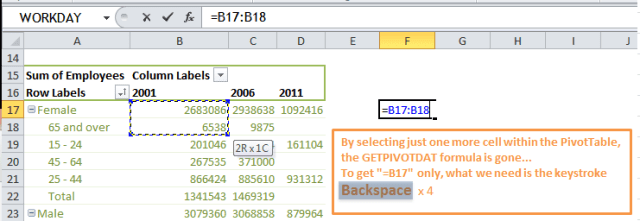

The GETPIVOTDATA formula will change to a simple range of two cells immediately.  What you need is just a few keystrokes of “Backspace”.

Try it out.

Note: If you have already released your mouse click, press Shift+Down Arrow, that has the same effect.

Wait… would it be easier to type =B17 directly? Yes, absolutely… provided that you did not point to the cell and generated the GETPIVOTDATA in the first place.  🙂