Christmas is all around.  Perhaps you are busy with decorating your Christmas tree with lots of joy.

However it’s no joy to decorate your Excel worksheets in your daily work.  It could be really time-consuming to apply the same set formats (note the “s”) into different tables.  What a repetitive and boring task!  If you have this feeling, there is a high chance that you do not know Format Painter, which is a very good assistance in Excel.  🙂

 Are you aware of this little icon (in Excel 2003 or before)?

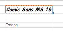
Just think about a cell in the following screenshot:

How many formats does it contain? Font size: 16 Bold Italic, Font Type: Comic Sans MS, Border: Solid, Outline… but not sure what color it is…  OK.  Let’s not take the color of the border into consideration for the moment.  If you need to apply this format to another cell, how many clicks are required?  TEN Clicks at least!!!!

With Format Painter, it takes you only three clicks!

First, click on the cell with the format you want.

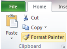
Second, click the Format Painter icon on the Ribbon (Home Tab) for Excel 2010

Third, with the Format Painter activated, click the cell you want to apply the format to

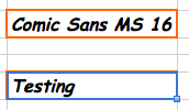
There you go!

This simple tool is one of my favorite assistances that helps apply consistent formats across different sections quickly.

Many users are disappointed that the Format Painter can only apply once.  Once the format is applied, the Format Painter is gone.  Then you have to click on the Format Painter again if you want to apply the same format to many different cells.  It’s just another repetitive and boring task…   Wait… have your ever hovered your mouse on the Format Painter and read the pop-up hint?

See!? If you wish to apply the format to multiples places, just double-click it so that you may apply the same format to different areas.  When you are done, press ESC.

Extra Hint: How to apply color band to alternative rows

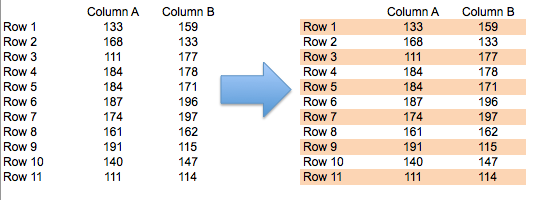
First: Apply the Color Fill on the first row of the table

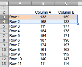
Second: Select the first two rows (the first one with color filled; the second one with no color filled)

Third: Click the Format Painter
  

Forth: Apply Format Painter to the rest of the table by dragging your mouse from 1st column 3rd row to last column and last row (i.e. A4:C13) of the table.

p.s. this can be easily done with Table (available in Excel 2007 or above)

Final step: Practice!