I think many people know how to AutoFit column width in Excel.  In case you don’t, you can simply move your cursor in between the column headers, when you see a cross with left-right arrow, double-click.  Then the column width will be adjust to fit the longest text string underneath the column.

However, AutoFit may not result in a nice-looking table as it gives you columns with inconsistent column width like the one below:

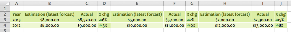
See, Column B and C are of different width because of the difference of the table headers.  Actually we want a consistent width for Column B and C, so we manually adjust it and have the following result (I have also make Column D a bit wider):

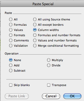
Then I want the rest of the table (Column E to J) follows the same width of Column B to D.  Instead of adjusting the column width one by one, we can use Copy, Paste Special -> Column Width:

1) Select any range from B:D, in this case B1:D1 is select, then COPY

2) Select any range from Column E to J, in this example, E1:J1 is selected, then Paste Special

3) Select “Column Width”

6) As simple as that.  Now you have consistent width throughout your table.

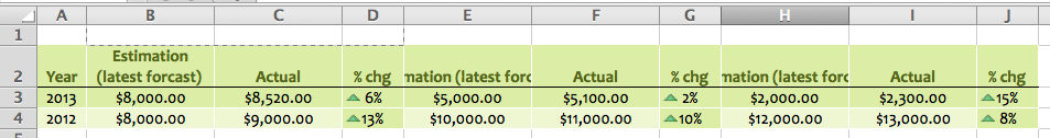
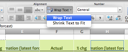
7) Now you just need to Wrap the Text in cell E2 and H2 to make it look nicer:

8) This is the final product

Hint: This could be very helpful when you copy and paste a well-formatted table to different columns as the Pasted table will follow the destination columns width.  You can do the pasting again with “Column Width” (You may refer to this blogpost for instruction).  It saves you time to adjust the columns width again and again… 🙂