Don’t get me wrong. I am not talking about the Filter button sitting on the Data Tab of ribbon,

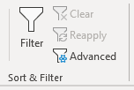
although they look almost exactly the same.

I am pretty sure that most people who use Excel five days a week is not aware of “AutoFilter”.

You may help strengthen/correct my understanding by a quick poll: 😁

Well, maybe you know about AutoFilter… but are you sure you know the “hidden” features of it?

There are two features, a standard one and a special one, of AutoFilter that I find really helpful. Let’s check it out.

You may download a sample file to follow along:

The standard one – Quickly filter a selected cell’s value

Think about the following scenario:

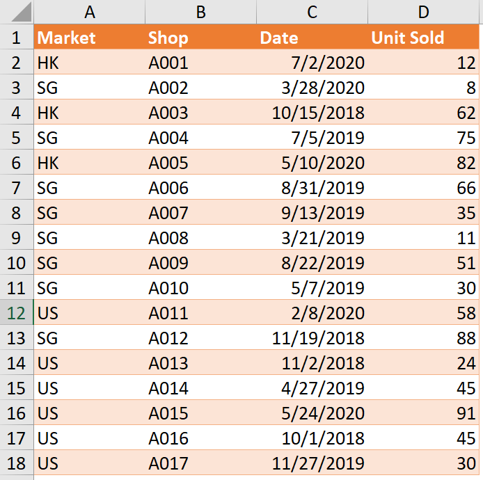
We want to filter records of “SG” market only. The common way to do it is

1. Apply Filter to the range of data
2. Filter by Market (by opening the pull down menu on the header of Market)
3. Select “SG”; then OK

Nothing special; and it’s not difficult at all. But what if, we can further streamline the process by fewer clicks?

Here comes AutoFilter to rescue!

With AutoFilter, we may simply select the cell that we would like to apply Filter to, then click the AutoFilter button. Just two simple clicks!

A picture tells a thousand words; a GIF tells even more. Let’s watch it in action. 😁

Isn’t it cool?

Indeed, we may achieve the same by right-clicking the cell -> Filter -> Filter by Selected Cell’s Value

If you are a keyboard person, check this out for the keyboard shortcuts.

Limitation:

This trick does not work on multiple range of selection; neither on multiple columns 😑

The special one – Quickly set a custom filter condition

Are you ready for an Excel magic?

Now imagine the following situation: Filter records with unit sold that is larger than 50.

You probably know the steps involved. We need to turn on filter, select “Number Filter” for “Unit Sold”, set the custom filter condition (which is larger than 50 in this example). Many steps (clicks) involved…

What if, we can simply input the condition (>50) at the end of the column, and then apply AutoFilter?

Sound too nice to be true? Let’s watch it in action:

Did you see that? The condition we input on D19 has been sent to the custom filter auto-magically. Isn’t it cool? 😎

Tips:

We may use < for less than, <= for less than or equal to, >= for larger than or equal to, <> for not equal to.

We may even use wildcards in setting up the custom condition.
For example: 
A* means begins with A;
*A means ends with A;
*A* means contains A

You may also be interested in my post: The proper way to filter values not equal to zero in #Excel

A drawback

Since we have literately input something at the end of the data range, it stays there. When we open the filter drop down, we will see it.

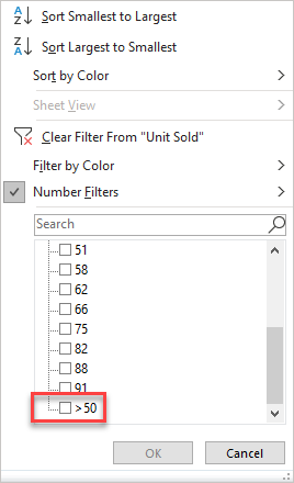
Remember to clear it afterward if you don’t need it in your dataset. 😵

Wait… so where is the AutoFilter after all?

It’s very hidden and we have to look it up.

First, click the last icon on your QAT (Quick Access Toolbar) -> Select More Commands

Then follow the steps below:

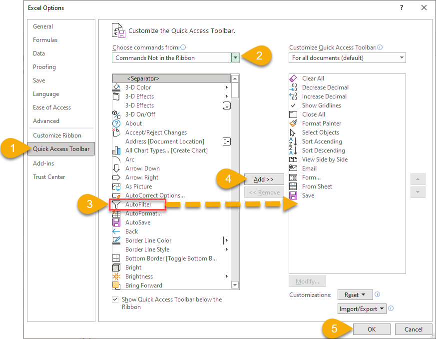
1. Quick Access Toolbar
2. Commands Not in the Ribbon
3. AutoFilter
4. Add->
5. OK

There you go! I hope you like it. 😉