Isn’t it nice?  Don’t think that this is difficult.  No VBA is required.  Indeed you only need to know a few Excel skills in order to create an interactive chart  with navigation panel like this.

The skills required:

1. Conditional formatting
2. A few functions: INDEX, ROW, basic logical test
3. Scroll bar
4. Create a bar chart (of course)
5. Linked picture (aka Camera)

That is all.

You may download the sample file to do “reverse engineering”, with the following hints.

How this is created?

Here’s how the raw data look like…

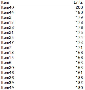
1) Do some makeup to the data

1. Turn the cell fill into grey;
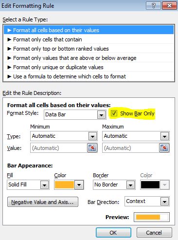
2. and convert the numeric data into bars by using conditional formatting.

This is the expected output:

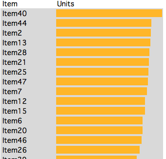
You will see why I turned the cells into grey in later steps…

Don’t know how to turn the numeric data into bar?

The following screencast shows you know to do it by conditional formatting in a few clicks:

Note: To show bar only, check the “Show Bar Only”.  

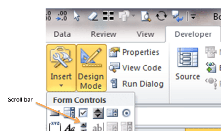
2) Insert a scroll bar

Go to Developer Tab –> Insert –> Scroll Bar (under Form Controls)

Once the scroll bar is inserted, right-click it to set the form control:

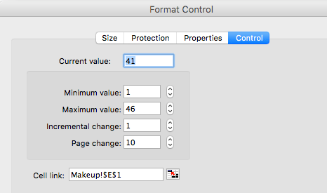
The setting is quite straight forward.  I leave it to you to explore on your own.  You will learn better by practising, even though trail and error sometimes.  Having said that, remind you that the Cell Link, and Min/Max values are crucial settings for what we are trying to do here.

In case the Developer Tab is not on your ribbon, do the following steps

1. Go to File Tab
2. Go to Customize Ribbon
3. Check the “Develop” on the right under Main Tabs
4. OK

3) More conditional formatting for the makeup

Again, I am not going to explain the rules set in details here.  I encourage to try it on your own.  The idea is to create visual effect, which depends on the value controlled by the scroll bar, to “highlight” only 5 items.

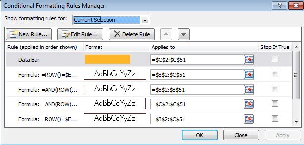
Hint: Do we remember we had set the cell fill to grey?  To have a “highlight” effect, we set rules to 

• No fill color  + surrounding border.

4) Make a “Linked Picture” ?

This is the trick to create the navigation panel.  A simple trick indeed.

A picture tells thousand words; a screencast tells even more: 🙂

Note: For demonstration, only a small range is selected in the above screencast.  You have to select the entire range where you want to take picture.

Related post: Paste Special – Linked Picture (aka “Camera” in earlier versions of Excel)

5) Set up a dynamic range of data for Interactive Bar chart

In cell I2, in our example, input:

=INDEX(B2:B52,$E$1) 'copy across and down to J6
where E1 is the linked cell of the scroll bar

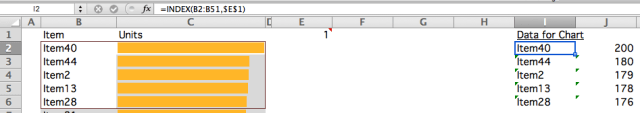
Question: Why do I not make absolute rows in the argument for INDEX?  🙂  (although it’s better to make it B2:B$52…)

6) Make a bar chart by using data in I2:J6

1. Select the range I2:J6
2. Insert Bar Chart (shortcut: Alt+F1)
3. Remove all the legend, title etc. (whatever you don’t need/like)

Note: Although it is commonly called “Interactive Chart“, the interactivity of the chart is actually governed by dynamic data – If the data is static, the chart is static; if the data is dynamic, the chart is dynamic.

7) Final Step: Tidy up

Put the three objects (the scroll bar, the linked picture and the bar chart) together nicely.

You may download the sample file to do “reverse engineering”.

Hope you like it.  🙂