A common VLOOKUP problem with an easy fix

The situation – VLOOKUP fails…

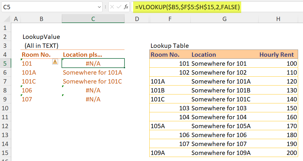
Have you ever encountered something like this? This is quite common. We are sure that the VLOOKUP formula is correct. We are sure that the lookup values are available in the lookup table (101, 106 107 in our example above). What we are not sure is the reason of the error returned… What happened?

The answer is simple: The “101” in B5 is different from the 101 in F5. What?? What’s the difference? The former is text, while the latter is numeric value. This is a basic but important concept for all Excel users, which I had discussed in the post HERE.

To fix the problem, we need to fix the data type in the lookup table. In other words, we need to make sure that all values for Room No. in the lookup table should be text (because the list of the lookup values in column B is text.

You may be wondering; can we simply change the cell format to text. See below:

Unfortunately, it does not work!

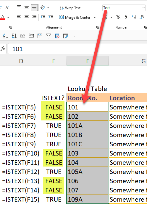
We cannot simply convert a number to text by changing the cell format. If we want Excel to accept a numeric input as text, we should set the cell format to Text BEFORE, not after the value is input.

We can use the function ISTEXT to test whether a value is text or not. See below:

Now we understand the problem. It’s time to show various solutions using formula approach. The trick is to use the function TRIM to convert all values under the lookup column into text to make the formula work.

You may download a sample file to follow along.

Let’s start with something simple, with a helper column.

Solution 1 – Helper Column

This would be the easiest way for and be welcomed by most users. Why is that? Because it is easy to execute and follow along. What is needed is a helper column next to the original lookup table. The goal is to convert all the values of Room no. into text. The function TRIM does the job.

In F5, input the following formula:

= TRIM(G5) 'Copy down

As you see in the following screenshot, we can construct the VLOOKUP formula as usual with the helper column. One thing we need to pay attention to is the new column index number (counting from the helper table).

And this is the formula input in C5:

= VLOOKUP($B5,$F$5:$I$15,3,FALSE)
'Note: the column index is 3 instead of 2

Solution 2 – VLOOKUP with TRIM

In some situations, we may not be able to add a helper column for whatever reason. If that’s the case, we can perform the VLOOKUP with a slight modification. And you won’t believe how simple the trick is.

This is the original formula that fails:

=VLOOKUP($B5,$G$5:$I$15,2,FALSE)

This is the modified formula that does the trick:

=VLOOKUP($B5,TRIM($G$5:$I$15),2,FALSE)

As you see, the trick is to wrap the lookup table with TRIM. The TRIM function here technically converts all values in the lookup table into text, and that is what we needed… even more than what we need. The following screenshot shows the new problem:

This modified formula works as along as the values to be returned are all text. In case we expect numeric values, it works only partially as all the results returned by the formula would be text. This is what we instructed Excel to do with TRIM.

Luckily, there is an easy fix. When we expect to return numeric values, we may modify the formula by adding two negative signs in front of VLOOKUP, as shown below.

In E5
= --VLOOKUP($B5,TRIM($G$5:$I$15),3,FALSE)
'Copy down

Wondering why? Please read the blogpost HERE.

As we have just seen, using VLOOKUP, and trimming the entire lookup table is not ideal. It would be nice if we could trim only the lookup keys. This is the moment we need solution 3 and 4. 😁😁

Solution 3 – XLOOKUP with TRIM

XLOOKUP is available in Microsoft 365 for Excel, and it is the perfect substitution of all existing lookup functions, in the future… because there are still quite a lot of users having no access to XLOOKUP. 😞

Talking about XLOOKUP, the arguments required is different from VLOOKUP. There are many differences which is not the key points in this post. What we need to know for this post is that the lookup table array and column index number are not required in XLOOKUP. Instead, we need to input the lookup array and the return array as the second and third arguments.

This arrangement makes the function much more flexible than VLOOKUP.

In C5, 
=XLOOKUP($B5,TRIM($G$5:$G$15),H$5:H$15)
'Copy down and right

Using the same trick of TRIM, the following formula works like a charm without the hassle of returning numbers as text.

Nevertheless, there is a high chance that we don’t have XLOOKUP (at work). No worries, INDEX and MATCH comes to rescue.

Solution 4 – INDEX and MATCH, with TRIM of course

There are lots of debates about which is better, VLOOKUP or INDEX and MATCH? It depends. Honestly in most scenarios, I use VLOOKUP simply because I am so getting used of it. Having said that, INDEX and MATCH wins in this situation as we can convert the lookup array instead of the entire lookup table.

Here’s the formula:

In C5,
=INDEX(H$5:H$15, MATCH($B5,TRIM($G$5:$G$15),0))
'Copy down and right

The logic behind is similar to the XLOOKUP. We specify the lookup array (inside MATCH) and the return array (inside INDEX) as two arguments, index column number is not required… just be reminded that the return array comes first in this construction.

Want to learn more about how this powerful combo work? Read the blogpost HERE.

Want to learn more about VLOOKUP? I have many blogposts about it. Check it out HERE. 😉

What do you think? Please leave your comments below.