When you are uncertain….. Draw a flowchart to decide!
A typical example of using Nested IF (unnecessarily) is to assign a grade to a test score, e.g.
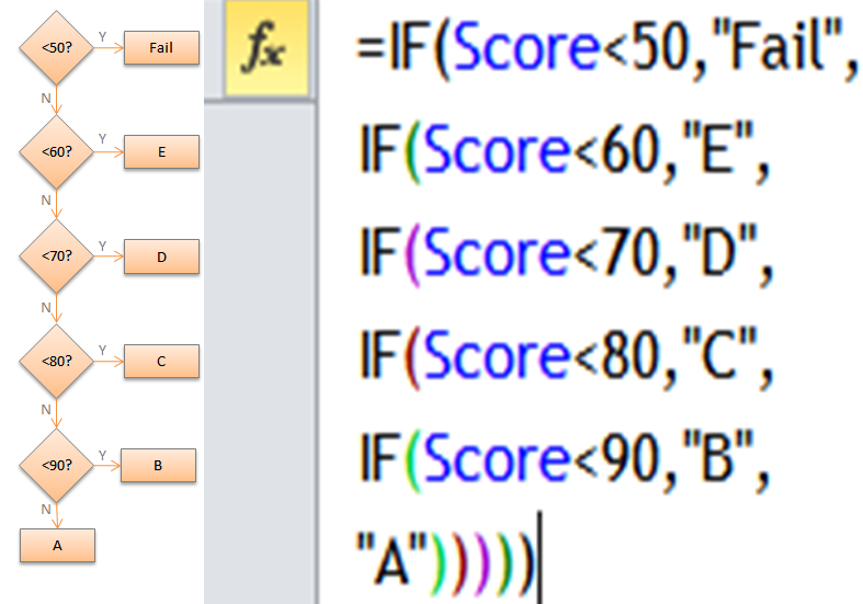
- below 50 –> Fail
- 50-59 –> E
- 60-69 –> D
- 70-79 –> C
- 80-89 –> B
- 90 or above –> A
This can be represented by a flowchart:

With the steps discussed in the previous post, the following nested IF formula can be constructed easily.
=IF(Score<50,"Fail",IF(Score<60,"E",IF(Score<70,"D",IF(Score<80,"C",IF(Score<90,"B","A")))))
Here’s a side-by-side image of the flowchart and the formula for better illustration:
Tip: It is a good idea to separate nested if statement line by line for better readability. To insert line break, press Alt+Enter whiling editing.
Try to practice nested IF on your own. It is not that difficult once you used to follow the flow of the chart.
Nevertheless, the same can be achieved with a much better formula:
=VLOOKUP(Score,tbl_Grade,2)
- where Score is lookup value;
- tbl_Grade is the lookup table for the grade, construct in the way as shown below:

- 2 is the column_index in this example as Grade is located on the 2nd column in the table while the lookup value (score) is on the 1st column
- The final argument of the VLOOKUP is omitted, meaning an approximate match
Notes:
- If you data type is categorical, e.g. red, green, blue etc, you may use VLOOKUP with exact match (False as the final argument) and you don’t have to care about the sorting order in the lookup table
- If you data type is real number, and you want to categorize the number, you may use VLOOKUP with approximate match (TRUE or omit the the final argument). Nevertheless, the data in the lookup data must be sorted in ascending order.
For more information of VLOOKUP with approximate match, please read HERE.
Now let’s take a look at our example used in previous post.
Can we use VLOOKUP instead of nested IF?
Yes we can, with the help of a a two-way table and MATCH function.
A two-way table below lays out the scenarios clearly.
With this table, we may construct the VLOOKUP with MATCH to solve the question:
=VLOOKUP(B3,$H$3:$J$4,MATCH(B2>=B1,$H$2:$J$2,0))

Is this formula above better than the nested IF below?
=IF(B2>=B1,IF(B3=0,"Good job","Serve better"),IF(B3=0,"Sell more","In trouble"))
Well, maybe… hmmmm…. not really…
Let’s wrap it up:
When we have one branch only in the flowchart, like the example we have in this post,
VLOOKUP
=VLOOKUP(Score,tbl_Grade,2)
vs.
Nested IF
=IF(Score<50,"Fail",IF(Score<60,"E",IF(Score<70,"D",IF(Score<80,"C",IF(Score<90,"B","A")))))
VLOOKUP wins!
When we have two branches in the flowchart, like the example in the previous post:

VLOOKUP
=VLOOKUP(B3,$H$3:$J$4,MATCH(B2>=B1,$H$2:$J$2,0))
vs.
Nested IF
=IF(B2>=B1,IF(B3=0,"Good job","Serve better"),IF(B3=0,"Sell more","In trouble"))
VLOOKUP wins in terms of length… However I can understand that you may prefer nested IF if you are a novel Excel user
Conclusion:
If your flowchart contains
- one branch only, use VLOOKUP (approximate or exact match according to your data type)
- two branches, consider 2D VLOOKUP (i.e. using MATCH for column_index) or Nested IF depending on your level of using functions
- three branches or more, consider nested IF (when there is no better alternative)
- whichever the case,
A well-drawn flowchart or a well-organized table helps you write a successful formula effectively


Good
LikeLike
Thanks. 🙂
LikeLike
Question
why are the formula are able to recognize that a grade falls in a range
namely 50 to 59
60 to 69
and so on
without having to enter that range into the formula
LikeLike
Hi David,
The tricky part is the final (optional) argument. When it is TRUE or 1 or omitted, it instructs Excel to perform an approximate match, assuming the first column of your data table is sorted in ascending order.
You may refer to the following site for more information.
https://support.office.com/en-us/article/Quick-Reference-Card-VLOOKUP-refresher-750fe2ed-a872-436f-92aa-36c17e53f2ee
LikeLike
A similar approach for these types of nested if..
=LOOKUP(Score,{0,50,60,70,80,90},{“Fail”,”E”,”D”,”C”,”B”,”A”})
LikeLike
Hi Deepak,
Thanks for your suggestion. LOOKUP a would do the same job as VLOOKUP does here.
Since we have already built the table of grade (tbl_Grade), we may use that instead of hard-coding it into the formula.
=LOOKUP(Score,tbl_Grade)
More flexible for modification, just in case. 🙂
LikeLike