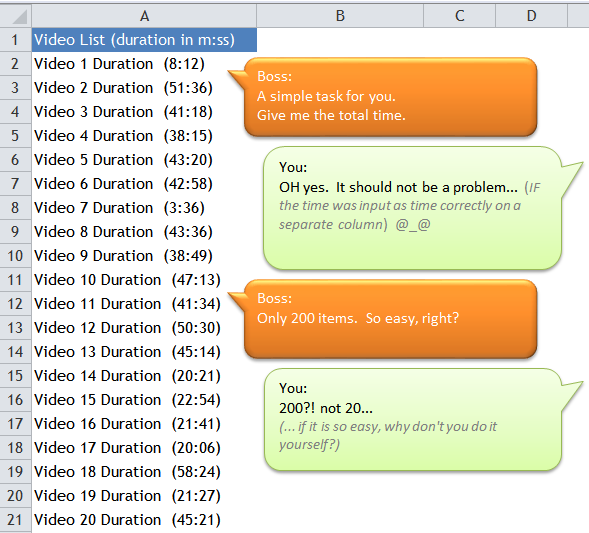
Did you encounter a task like this?  I did.  Actually it is not as difficult as you may expect.  It could be done in just a minute IF the data is not too bad, like the one shown above.

I am going to show you two approaches to handle this:

1. Formula;
2. A combination of simple techniques that even a regular Excel user should be able to manage.

1) Formula Approach

 =SUMPRODUCT(("0:"&SUBSTITUTE(SUBSTITUTE(RIGHT(A2:A21,6),"(",""),")",""))+0)

Let’s examine it inside out.

 RIGHT(A2:A21,6)

Since we are so lucky that the time we need are all sitting in the end of a text string, enclosed by (),  we may use RIGHT(A2:A21,6) to extract the time portion from the text string.  And this is the resulting array:

{"(8:12)";"51:36)";"41:18)";"38:15)";"43:20)";"42:58)";"(3:36)";"43:36)";"38:49)";"47:13)";"41:34)";"50:30)";"45:14)";"20:21)";"22:54)";"21:41)";"20:06)";"58:24)";"21:27)";"45:21)"}

Because the time is in m:ss format, there are cases of “(” being extracted.  Thus we need to

Remove both “(” and “)” from the array by using SUBSTITUTE(text, old text, new text)

 SUBSTITUTE(SUBSTITUTE(RIGHT(A2:A21,6),"(",""),")","")

The result then becomes:

{"8:12";"51:36";"41:18";"38:15";"43:20";"42:58";"3:36";"43:36";"38:49";"47:13";"41:34";"50:30";"45:14";"20:21";"22:54";"21:41";"20:06";"58:24";"21:27";"45:21"}

which is very close to what we need…

Concatenate “0:” (zero colon) to the resulting array

 ("0:"&SUBSTITUTE(SUBSTITUTE(RIGHT(A2:A21,6),"(",""),")",""))

As Excel would interpret the result as hh:mm we need to concatenate “0:” to the above array to make sure that the resulting time will be interpret correctly as mm:ss.

{"0:8:12";"0:51:36";"0:41:18";"0:38:15";"0:43:20";"0:42:58";"0:3:36";"0:43:36";"0:38:49";"0:47:13";"0:41:34";"0:50:30";"0:45:14";"0:20:21";"0:22:54";"0:21:41";"0:20:06";"0:58:24";"0:21:27";"0:45:21"}

Adding 0 to the above result to convert the text into a real time value

 ("0:"&SUBSTITUTE(SUBSTITUTE(RIGHT(A2:A21,6),"(",""),")",""))+0

Results in:

{0.00569444444444444;0.0358333333333333;0.0286805555555556;0.0265625;0.0300925925925926;0.029837962962963;0.0025;0.0302777777777778;0.0269560185185185;0.0327893518518519;0.0288657407407407;0.0350694444444444;0.031412037037037;0.0141319444444444;0.0159027777777778;0.0150578703703704;0.0139583333333333;0.0405555555555556;0.0148958333333333;0.0314930555555556}

Feeding the array into SUMPRODUCT to give the total

i.e. 0.49056712962963 or 11:46:25 (format as [h]:mm:ss)

Not really difficult… 🙂

If you are good in using FUNCTIONS and know about array formulation, it should not be too difficult.  Nevertheless, I know that there are quite a lot people using Excel are having Formula-phobia.  😛  That’s why I am going to show you an non-formula approach, which may be even faster.

2) Non-formula approach.

Copy another set of your data and paste it on the next column

Using Find and Replace to get the time portion (tip: CTRL+H to open the Find and Replace dialog box.  Note: Select the range you want to perform Find and Replace beforehand, otherwise your original data will be in danger…)

• First Find *( and Replace with 00:

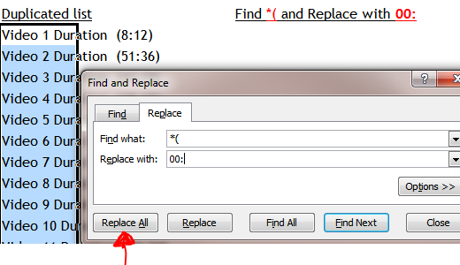
• See the changes?!  Then Find ) and Replace with nothing

• Now you should have the time portion extracted properly:

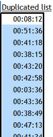(You may format it back to mm:ss if required)

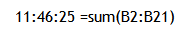
A simple SUM would do the rest

Did you notice that the above steps are actually the same as the ones described for formula-approach?!

Here’s a Sample File file for you to download.

Honestly, if it is an one-off task, I would absolutely do it in the way demonstrated in the 2nd approach.  How about you?