4 different ways to perform LOOKUP with 2 lookup values
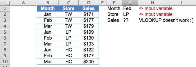
We know that VLOOKUP is very useful. At the same time, we know that VLOOKUP has its limitations. E.g. VLOOKUP only looks from left to right; VLOOKUP only handle one lookup value. For a simple situation shown below, VLOOKUP doesn’t seem to work (directly).

No worry. There are at least four workarounds!
- Using a helper column
- Using CHOOSE to recreate the Table Array for VLOOKUP
- Using INDEX, MATCH and = Operator
- Using SUMPRODUCT
Let’s start with the basic.
1. Using a helper column
Most of the time, complicated problem will become easier and manageable when it is broken down into small pieces. Same applies in formula building in Excel.
Take below example:

By CONCATENATING “Month” and “Store” in column A (note: better to put the helper column to the left of the original Table as VLOOKUP looks from left to right.), we create the lookup value required in column A. As a result, with the helper column A (which could be hidden later), the problem can be solved easily by
=VLOOKUP(G1&G2,$A$2:$D$10,4,FALSE)
Note: we need to combine the Month (G1) and Store (G2) as the lookup value
Non-helper column approach
Well, for any reason a helper column is not an option, we may do it by array formula. At least two different ways to perform the job:

2) Using CHOOSE to recreate the Table Array for VLOOKUP
This is a bit advance. The tricky part is to re-create the Table Array that is suitable for VLOOKUP by using CHOOSE.
CHOOSE({1,2},B2:B10&C2:C10,D2:D10) does two things
- Combine “Month” and “Store” into a single array as “JanTW”;”FebTW”, etc……
- Join the two arrays into a “table” of two columns
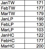
When we evaluate the result of the above CHOOSE (by selecting the whole CHOOSE formula in the formula bar and then press F9, we get the following result:
{"JanTW",171;"FebTW",177;"MarTW",179;"JanLP",199;"FebLP",130;"MarLP",103;"JanHC",122;"FebHC",177;"MarHC",200}
To visualize it in a Table format, it looks like the below:

Now the whole formula makes sense:
=VLOOKUP(G1&G2,CHOOSE({1,2},B2:B10&C2:C10,D2:D10),2,FALSE)
 CTRL SHIFT ENTER (not just ENTER)
IMPORTANT: As this is an array formula, we have to input CTRL SHIFT ENTER to tell Excel that we are going to input array formula. You will see the {} in the formula bar if array formula is input successfully.
-
- Note: For both 1) and 2), the robust way to combine the lookup values should include a delimiter in between, e.g. A1 & “|” & B1 . Please read Pay attention when concatenate for explanation.
3) Using INDEX, MATCH and = Operator
=INDEX(D2:D10,MATCH(1,(B2:B10=G1)*(C2:C10=G2),0))
 CTRL SHIFT ENTER
This formula actually looks more intuitive. How?
First let’s understand what the (B2:B10=G1)*(C2:C10=G2) does?
- B2:B10=G1 asks Excel to evaluate if B2=G1, if yes, it returns TRUE; if no, it returns FALSE. Then do the same for B3=G1, B4=G1…… until B10=G1. An array of TRUE/FALSE will be the result.
- C2:C10=G2 basically does the same thing but look at different values.
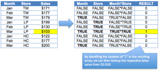
When we compare the two array of TRUE/FALSE by multiplying them, only TRUE * TRUE gives the result of 1 (TRUE). A picture tells more. Let’s take a look at the screenshot below:

Bingo, we can identify the row that meets both lookup values.
Now you should be able to use MATCH to identify the position of the matching values. Then use INDEX to return the result required.
- =INDEX(D2:D10,MATCH(1,(B2:B10=G1)*(C2:C10=G2),0)) gives
- =INDEX(D2:D10,MATCH(1,{0;0;0;0;0;1;0;0;0},0) gives
- =INDEX(D2:D10,6) returns
- $103, the correct result!
4) Using SUMPRODUCT
SUMPRODUCT is a powerful function in Excel. I am going to write separate posts about SUMPRODUCT later. Although SUMPRODUCT seems to work in our example, it actually fails if the result we want is text instead of value.

To understand that, we have to understand how SUMPRODUCT behaves. If you want to know more about SUMPRODUCT, stay tuned! 🙂
So, which one do I use?
Although options 2) and 3) works fine, I prefer option 1) under normal circumstance. Why?
In daily work life, I believe it is more important to build a spreadsheet that is manageable and readable by most users (including myself)… Not every one in workplace is Excel guru. If every one is, we don’t have to spend so much time to fight with spreadsheets.
As such, let’s obey the KISS principle whenever possible.


Hi to every one, the contents existing at this site are actually remarkable for
people knowledge, well, keep up the good work fellows.
LikeLike
Thank you very much. Glad that you find this site helpful to you and others. 😀
LikeLike
Hi all
=vlookup(A2&B2,….. WILL WORK FOR BELOW
Custom DEC No. Country Of Origin Quantity PCS Total Weight Total AMOUNT
3020401577416 THAILAND 10 3.26 31.8
3020404560816 JAPAN 10 7.18 47.898
3020404560816 THAILAND 1 1.053 5.535
I NEED TO CHECK WITH TWO COLUMN……FIRST AND SECONF
LikeLike
Hi,
I tried using your “index match =” method on excel 2016 and it doesn’t work. I recreated your spreadsheet, and it still wouldn’t work.
The result is always #N/A.
I used the “show calculation steps” button and it showed me how it took the values and compared them with each other but got false and it never continued afterwards. How do I make sure even if the values don’t match at first, excel would continue down the range?
Could you please help?
LikeLike
Hi Jason,
That is an array formula and require Ctrl+Shift+Enter.
Hope it helps.
LikeLike
i want to combine the formulas below into one
(B2)-> VLOOKUP(A2,BASS,2,FALSE)
(b3)->VLOOKUP(A2,BASS,3,FALSE)
B4-> IF(AND(B2=”S”,B3=”M”,”YES”,”NO”)
LikeLike
Hi ram, you have the formula you need already, just need to combine it carefully.
Pls read below post for your reference
Writing a long formula in steps | wmfexcel
LikeLike
Thanks for the wonderful explanation. it works great!!
LikeLike
Glad it helps! 😄
LikeLike
Just wanted to say thank you!
LikeLike
You are welcome!
LikeLike
Thank you very much for your tips, sure i will follow your tips.
For more information: http://www.labstech.org/tutorial-excel-tips-and-tricks-2013-09-03/
LikeLike
Pingback: Multiple Lookup based on FirstName LastName to return Phone number
Hi
Really liked idea of using choose, but sumproduct would fail if there is multiple matching items..
Cheers!!
ExcelVbaLab.Com
LikeLike
Glad you like it.
If there is multiple matched records, none of the above would work as they will return the first matched record, like VLOOKUP does.
So we need to be careful and really study the data first.
Cheers,
LikeLike
Hi Fung,
Like you said below – “VLOOKUP will return the first matched value found” or above, in case there are multiple matched records what formula should we use? Maybe Index+Match will work better?
LikeLike
Hi Igor,
If you need to lookup multiple matched records, VLOOKUP is not the function you are looking for. Indeed, there is no simple function to achieve that. We need a combination of functions and array formulation.
As a simple alternative, you may consider using an extra helper column to identify the incidence of occurrence for an item. The formula would be =COUNTIF($C$2:C2,C2) when we refer to example 1 in this post.
With that helper column, we can then concatenate the number with the lookup item and deploy the method we described example 1.
You raised a very good question and I will put it on my list and write a post in the future.
Cheers,
LikeLike
Thanks, will wait for your study on this topic.
P.S. I checked Index+Match doesn’t work. Same as Vlookup those two returning only first matched record. In my case I can’t use something like SUMIF, as I’m looking for employee’s rate, which can’t be combined. I differently need something different if array has more than one unique value.
LikeLike
Also want to add – if Using a helper column we can use this formula:
=SUMIF(A2:D10,G1&G2,D2:D10). Without helper column we can use this formula: =SUMIFS(D2:D10,B2:B10,G1,C2:C10,G2)
LikeLike
just to remind, it works only when
1) there are no duplicates;
2) the result you expected is number, not text.
LikeLike
Hi MF!
I can’t understand about CHOOSE function in array formula.. Why do we have to use choose? Would u explain it in simple way? Thank you very much 🙂
LikeLiked by 1 person
Hi Andrewsipahuta,
You gave me a challenging question: to answer it in a simple way… 😛
I will try my best:
First you need to understand what CHOOSE does.
The syntax:
CHOOSE(index_num,value1,value2,…)
Depends on the index number, it returns the corresponding value from a list of values you feed into the function. For example:
=CHOOSE(1,”A”,”X”) returns “A”
=CHOOSE(2,”A”,”X”) returns “X”
=CHOOSE({1,2},”A”,”X”) returns an array of “A”,”X”
To go a bit further,
=CHOOSE({1,2},{“A”;”B”;”C”},{“X”;”Y”;”Z”}) returns an array of {“A”,”X”;”B”,”Y”;”C”,”Z”}
So basically it “re-construct” a table_array with two columns:
“A”,”X”;
“B”,”Y”;
“C”,”Z”
Now going back to our example in the post, “Month” and “Store” are concatenated into a single array. And we need CHOOSE to “re-construct” the Table_array required for VLOOKUP.
Hope you can understand it better now.
Cheers,
LikeLiked by 1 person
Hi MF!
I understand now.. So, we proposing “a new array” with Choose({1,2},…. Rather than “choosed” from (“A” & “X”), we selected both columns with that function then vlookup the value from the “new array”.
Thank you for your explanation, it’s been clear in a simple way 😀
LikeLiked by 1 person
You are welcome! Glad it helps 😀
LikeLike
Pingback: Hlookup with two conditions?
hi. tks for your info,, 😀
LikeLike
Hi nadia
You are welcome! 😄
LikeLike
Is it possible to get sales only by using vlookup function Eg: G3 =vlookup(G2,D2:D10,3,FALSE) =vlookup(G1,C2:C10,2,FALSE)
LikeLike
Hi Saurabh,
Your formula is actually comparing the results returned by two VLOOKUPs. You will likely get a result of “FALSE”.
If you need to lookup two values, the above examples should do the job.
On the other hand, remind you that if you are looking up single value only, you should check if there are duplicates in your Table VLOOKUP will return the first matched value found. You may refer to my post regarding vlookup for more information.
LikeLike
Hi I’m trying to do this but using different worksheets and a dropdown option. I tried doing the 3rd option but still having trouble. Would you care to suggest what can be done please?
Here’s the link to my inquiry on reddit:
Thanks so much!
LikeLike
Hi Amy,
IF you end up with #NAME, that means your Named Range or Functions used in your formula do not exist, most likely being mis-spelt. Please check.
Cheers,
LikeLike
If you are interested in learning How to Use Vlookup Function without using Helper Column
http://www.exceltip.com/tips/how-to-use-vlookup-function-without-using-helper-column-in-microsoft-excel.html
LikeLike
Hi ashish,
Thanks for sharing the article.
I believe I have also captured the content in this post. I would suggest you to take a look at my another post “Pay attention when concatenate” when you are using CHOOSE with & in order to perform to vlookup.
Here’s the link for your reference.
https://wmfexcel.wordpress.com/2014/05/11/perform-vlookup-with-2-lookup-values-2/comment-page-1/#comment-484
Cheers,
LikeLike
Plz upload an example file for all above formulae
LikeLike
Hi Hayat,
Thanks for your suggestion. The truth is… I don’t know how to upload sample file here. 😛
On the other hand, I suggest you input some simple data and follow the steps shown above. In this way, although it may take longer time and more effort, you will learn better as you go through the whole process on your own.
Cheers,
LikeLike
Pingback: Note lookup with 2 conditions
Pingback: Two criteria for a lookup table
Pingback: 3 Way Lookup By splitting the Cell value